Project 2
Fun with Filters and Frequencies
Fun with Filters and Frequencies

In this project, we explore two apparently unrelated concepts - filters and frequency!
As we progress through this project, we will see that these are actually closely related ideas.
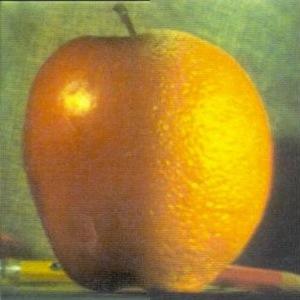
My recreation of orapple
Sometimes we want a way of quantifying where the largest changes in the image are happening. If images were continuous, we might consider taking the derivative. However, since an image is discrete, the best we can do is take a delta between pixel values over a specified period.
One way of doing this is through the Finite Difference Operator. By convolving the image with the mask [1, -1], we get a new matrix representing the deltas in the horizontal direction. We can do a similar thing with its transpose to get the differences in the y direction.
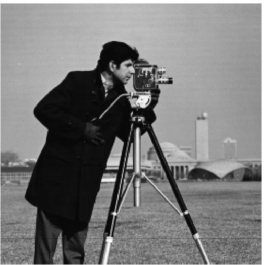 Original Image
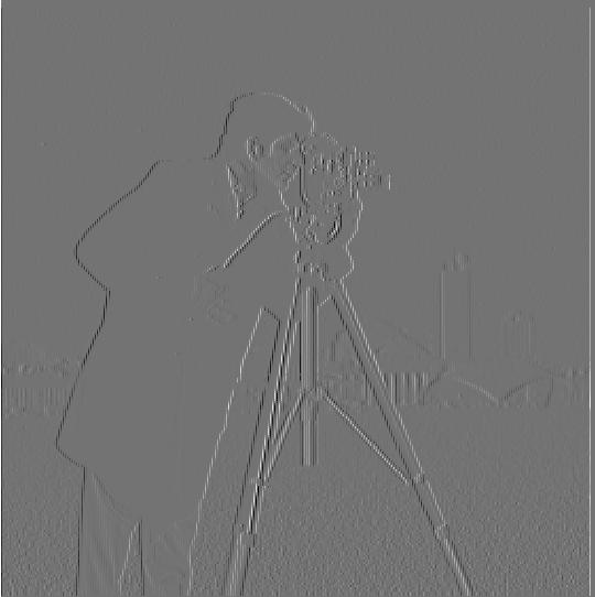 dx
dx
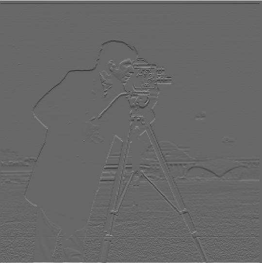 dy
dy
By taking the pixel-wise gradient magnitude using the two masks from the last step, we can produce a gradient magnitude image, which represents the discrete gradient at every point in the image.
Lastly, we may find it useful to assign a cutoff frequency to the gradient magnitude image produce an edge image with only 2 states: 255 for an edge, 0 for not an edge.
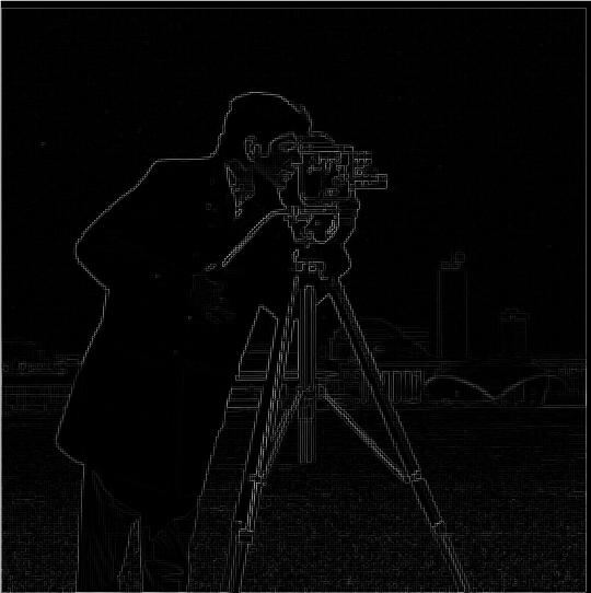
Gradient Magnitude Image
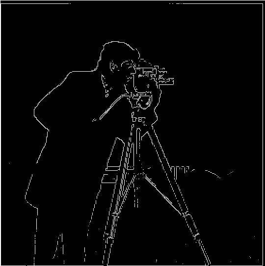
Edge Image
The filter is effective at outlining strong edges such as the man against the sky and the tripod, while cutting out irrelevant noise, such as blades of grass.
Often, very small localized areas of change can erroneously be misclassified as edges. Additionally, you can see areas in the man's coat above where the edge is very thin or even broken in places. It would be better if our edge detection method was a little more robust to noise.
We can use a gaussian filter to blur the image, which will reduce the effect of very localized noise:
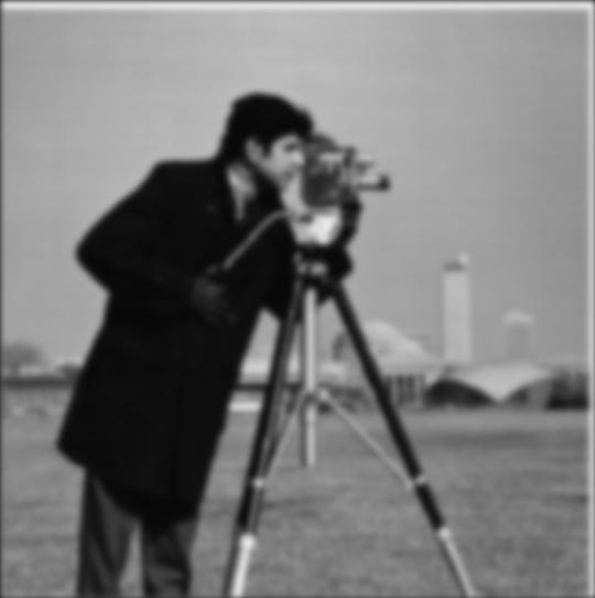
Gaussian blur applied to original image
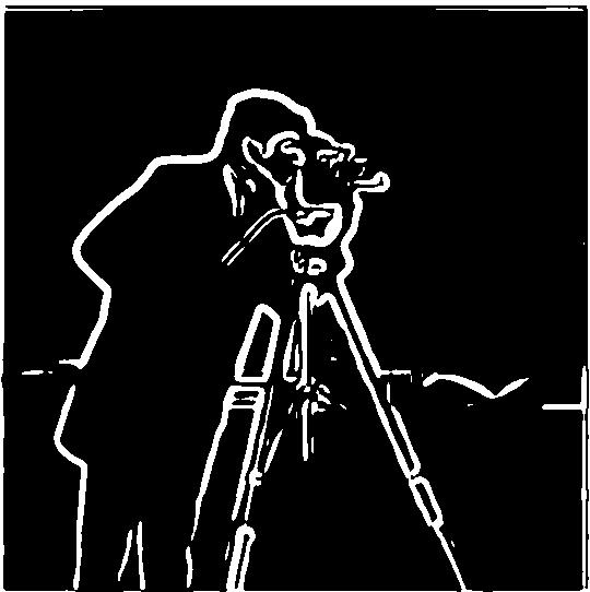
Edge detection applied to blurred image
Now we can see that the edges are much more thick and robust compared to the original edge image. The only place where the man's coat is not highlighted as an edge is where the background blends perfectly into it, such as the bottom left corner of his coat. There are very few false positives.
There is one last modification we can make to create the Derivative of Gaussian filter. Because convolution is a commutative operation, we can apply the gaussian blur directly to the dx and dy filters. It is more efficent to do it this way, as applying a convolution to the smaller dx and dy filters is much cheaper than convolving with the (potentially very large) image.
The x and y DoG Filters, as well as the result of using them for edge detection, is below.
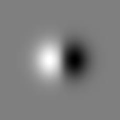
X direction DoG
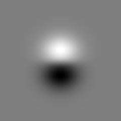
Y Direction DoG
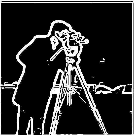
Result of using DoG for edge detection - identical to the image from above
If gaussian filters work blur images, and they work as a low pass filter, then it is intuitive that subtracting the result of a gaussian filter from an image acts as a high pass.
Adding these high frequencies back to the image can make it appear "sharper". We call this the unsharp mask filter. The k value below represents what multiplicative factor we used when adding these frequencies to the original image.
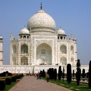
k = 0 (Original)
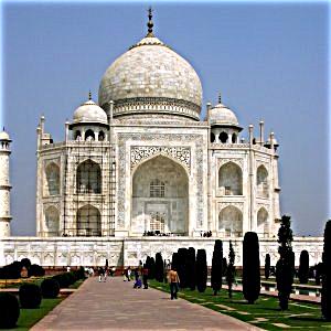
k = 1
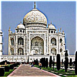
k = 5
For this image, it worked reasonably well. You could argue that the k = 1 image looks better than the original.
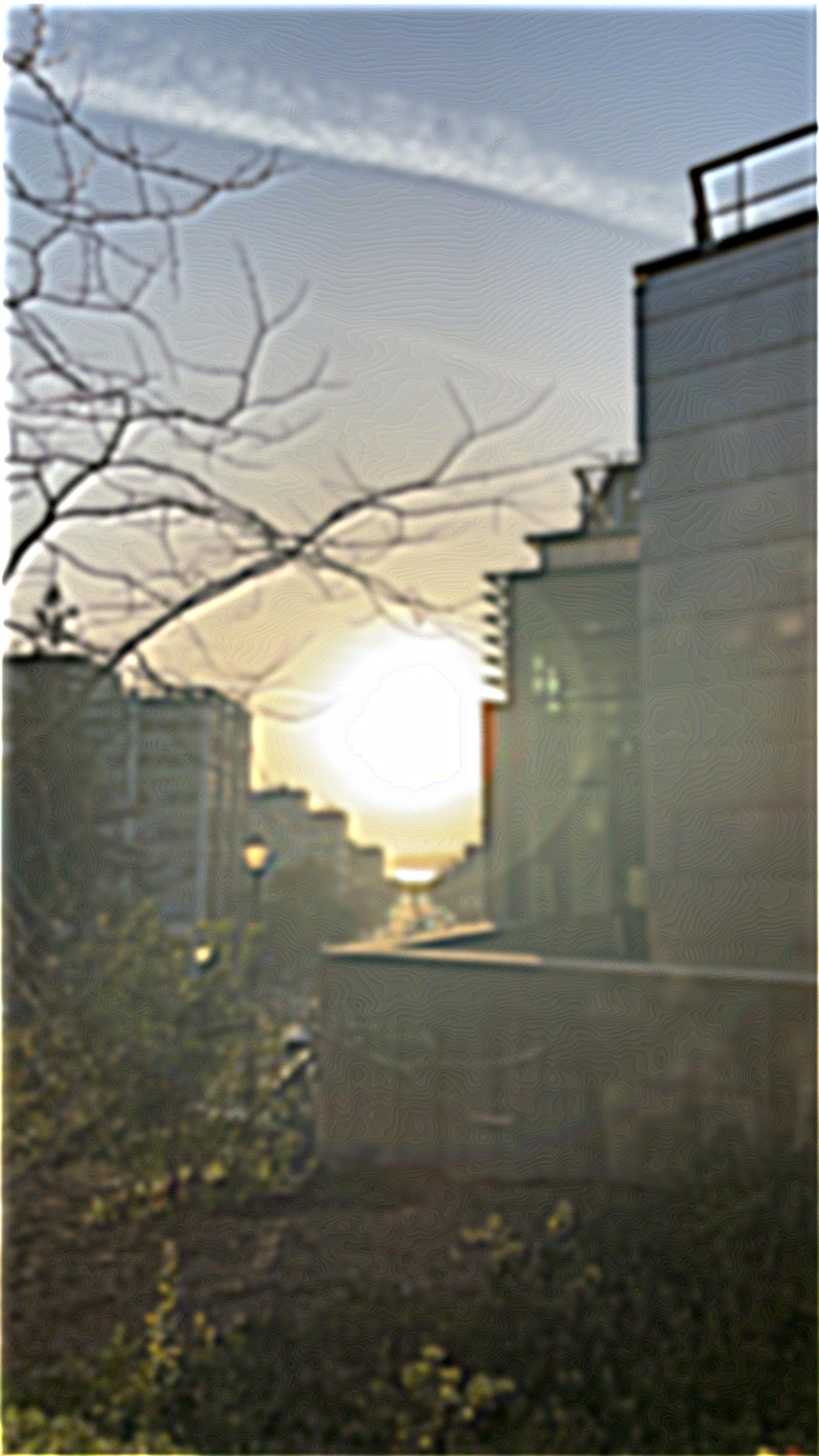
Now, lets try adding our own blur, and then attempt to recover the image.
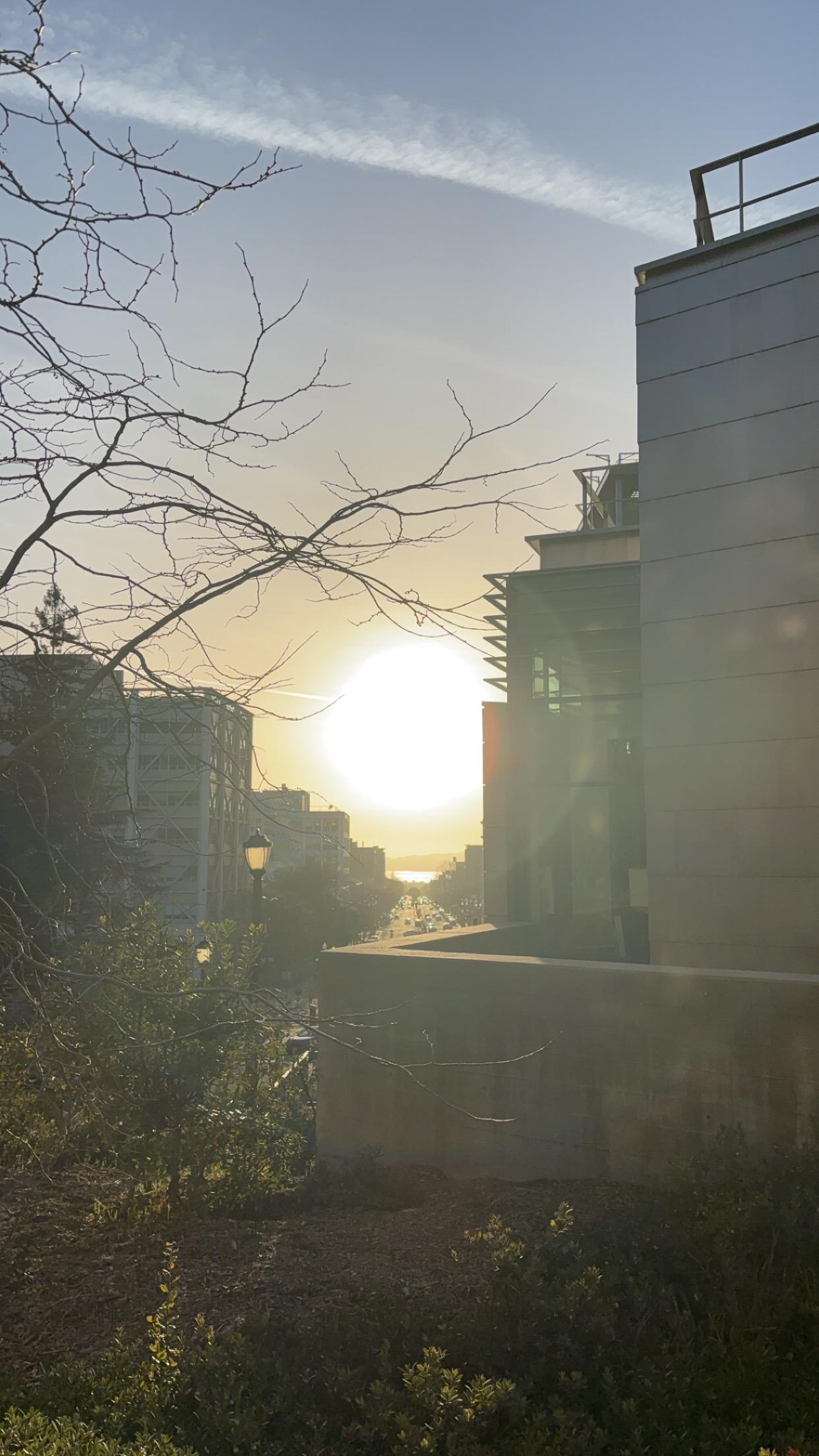
Original

Blurred
Restored
For this image, it also works ok. You can make out a little more detail in the restored image than the blurred one, particularly in the leaves on the tree, but it is far from perfect.
k=0 (Original)
k=1

k = 5
For this image, the unsharp mask filter was not very effective. Even the k = 5 image is still very blurry, yet it is even more uncomfortable to look at. The unsharp mask filter is definently not magic.
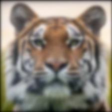
By adjusting cutoff frequencies, it is possible to merge 2 images together such that it looks like one image up close, and a different image from further away. This is because the high frequencies dominate when visible, but as the viewer looses the ability to make out the fine details, the low frequencies appear. Therefore, by averaging the result of a low pass filter on one image and a high pass on another, you can create a hybrid image.
If you have trouble seeing the result, try openning the image in a new tab and zooming in and out.
Tiger (Low Pass)
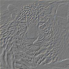
Jaguar (High Pass)
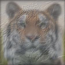
Tiguar (Hybrid Image)
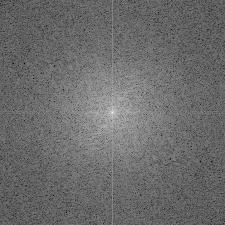 Jaguar
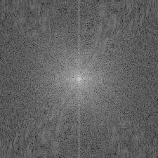 Tiger
Tiger
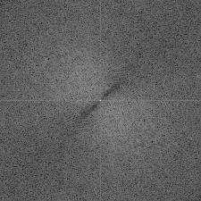 Jaguar Filtered
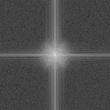 Tiger Filtered
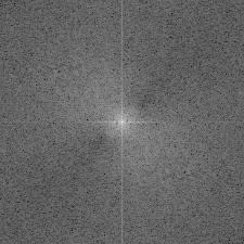 Hybrid Image
Smiley (Low Pass)
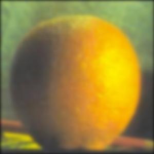
Orange (High Pass)
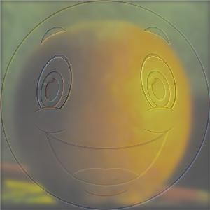
Smorange (Hybrid Image)
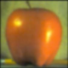
Apple (Low Pass)

Another Apple (High Pass)
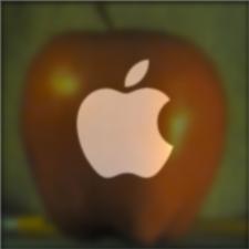
Apple ^ 2 (Hybrid Image)
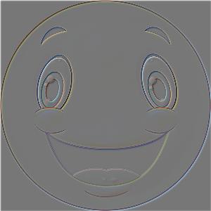
Laplacian stacks are a way of seperating an image's frequencies into different layers. They are a prerequisite to the blending we will do in the next section.
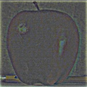 Level 1
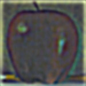 Level 2
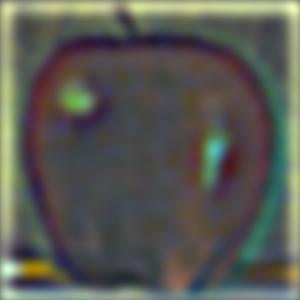 Level 3
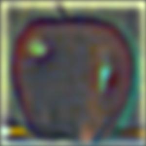 Level 4
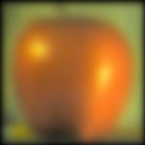 Level 5 / Bottom of gaussian stack
 Reconstructed Apple - 5 previous levels summed together
 Level 1
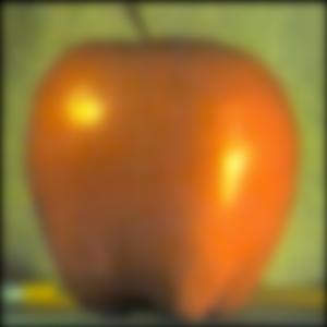 Level 2
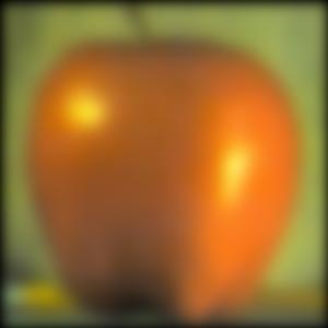 Level 3
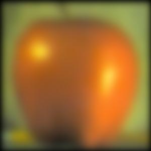 Level 4
 Level 5
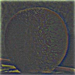 Level 1
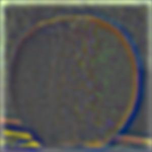 Level 2
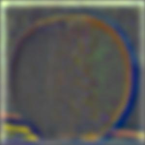 Level 3
 Level 4
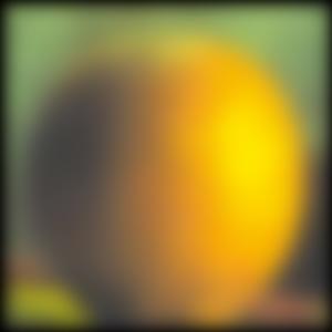 Level 5 / Bottom of Gaussian Stack
 Reconstructed Orange - 5 previous levels summed together
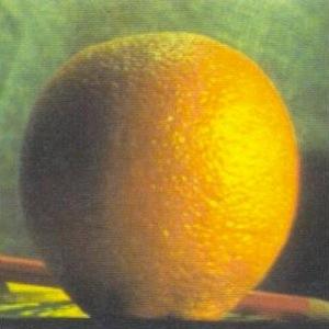 Level 1
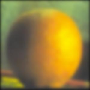 Level 2
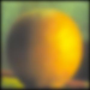 Level 3
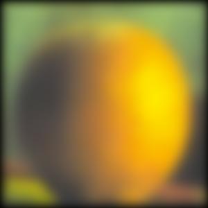 Level 4
 Level 5
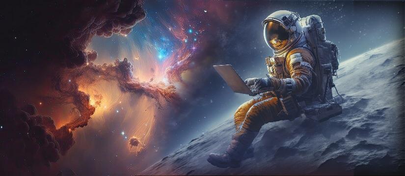
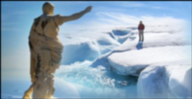
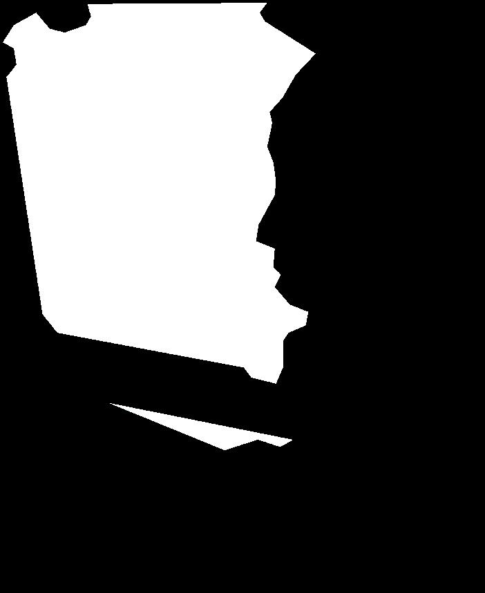
Sometimes, we would like to merge images together so they look coherent. However, as you can see below in the space image, simply stitching the images together makes the seam very apparent.
Instead, we can do something called multiresolution blending. The key idea is that we can blend frequencies between the images at different rates - so high frequencies are less blurred than low frequencies. This retains the structure of both images, while tricking the eye into beleiving they look coherent.
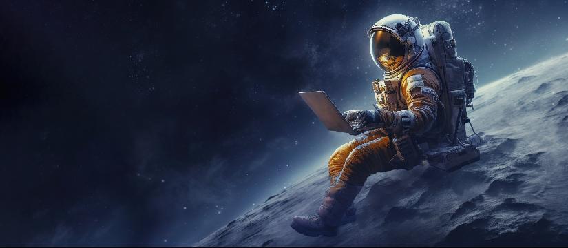 Image 1
 Image 2
 Filter
 No Blending
 Multiresolution Blending
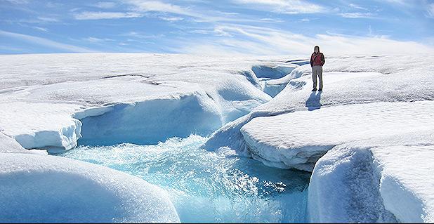 Image 1
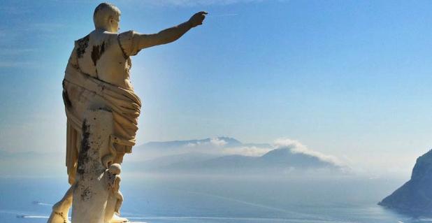 Image 2
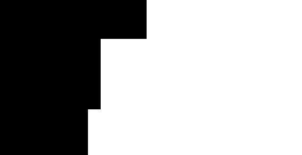 Filter
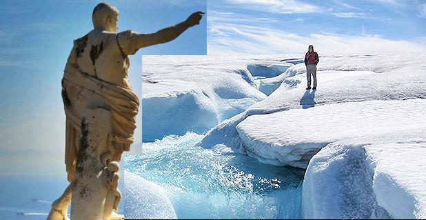 No Blending
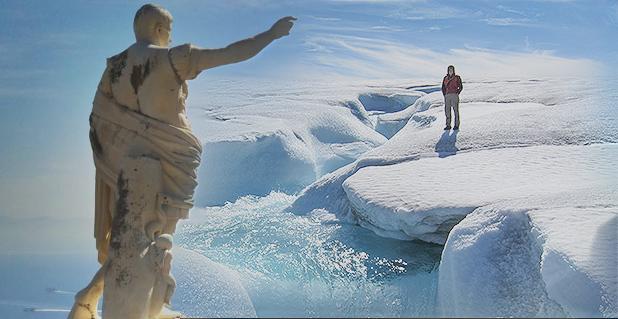 Multiresolution Blending
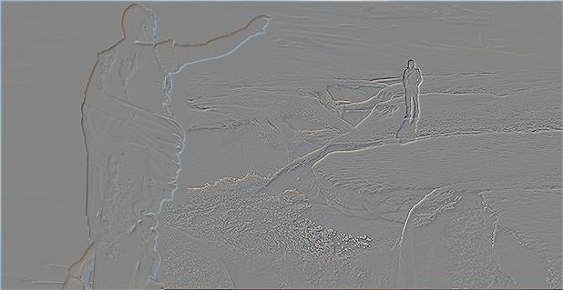 Layer 1
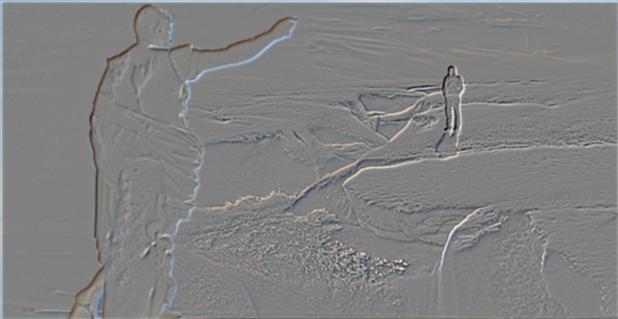 Layer 2
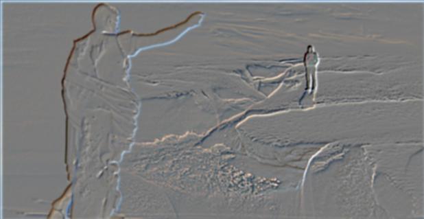 Layer 3
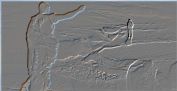 Layer 4
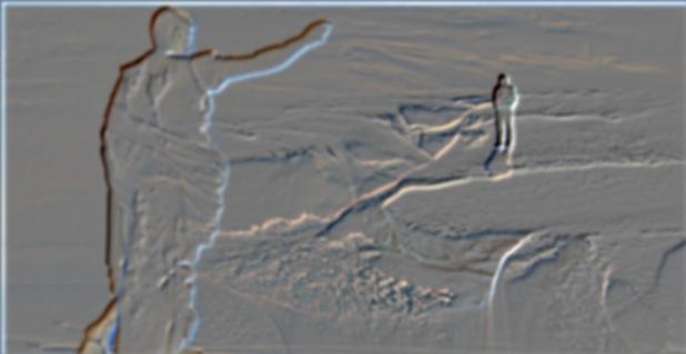 Layer 5
 Layer 6
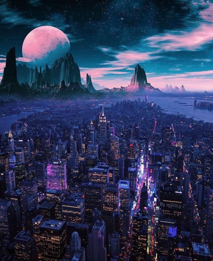 Image 1
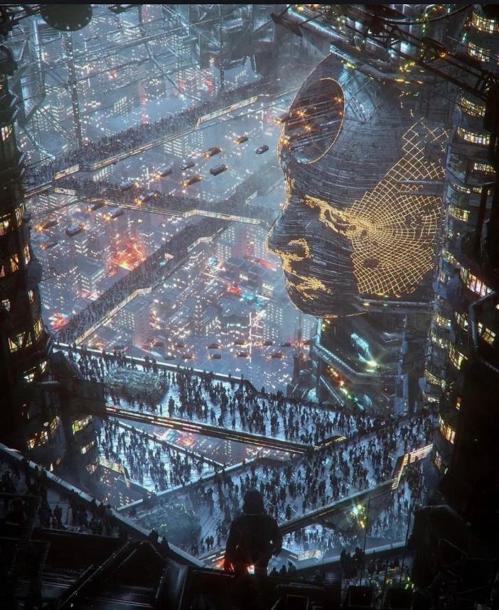 Image 2
 Filter
 No Blending
 Multiresolution Blending