Project 4
Image Warping and Mosaicing
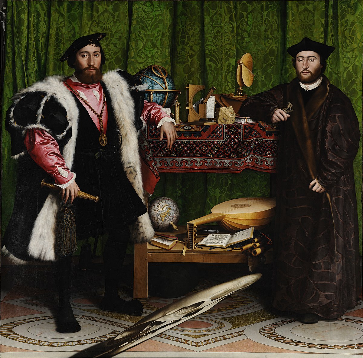
Image Warping and Mosaicing

In part 1 of this project, we explore how images taken from one perspective can be warped to appear as if they are being viewed from a different perspective. This also allows us to create mosaics of multiple images cobbled together.
In part 2 of this project, we will figure out how we can make this process automatic. While in part 1, we will tell the computer which parts of the overlapping images correspond to each other, in part 2 we will get the computer to do this itself. We will follow the paper "Multi-Image Matching using Multi-Scale Oriented Patches" by Brown et al.
The subtle skull rectified from Holbein's painting "The Ambassadors" to its intended viewing angle
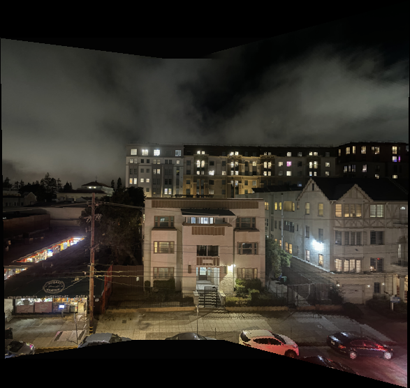
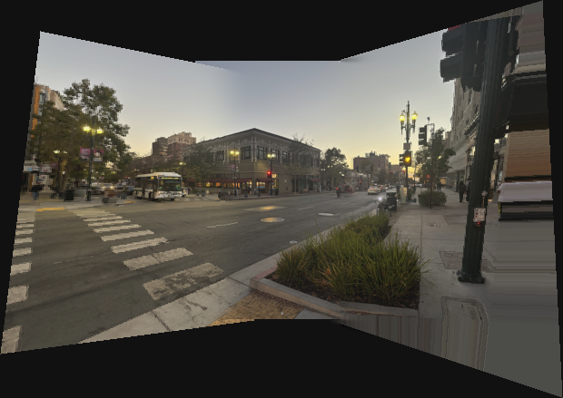
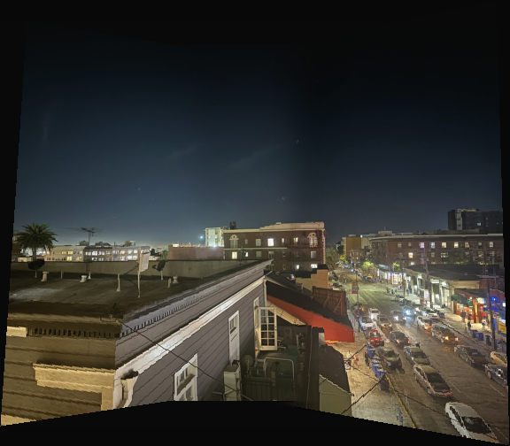
Here are the three sets of pictures that I will want to unify into three images by the end of the project:
A homography, or projective transformation is a distortion of space with 8 degrees of freedom. It is more powerful than a linear transformation as it does not necessarily preserve parallel lines. However, straight lines remain straight after the transformation is applied.
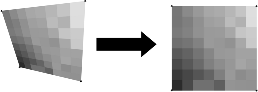
An example of a perspective transformation (homography)
In the graphic above, notice how it looks like you are looking at the left polygon from slightly up and to the right - this is why it is called a perspective transformation. Since our goal is to modify the perspective of the images, this is the transformation we want.
Perspective transformations are simply to calculate given 4 points (corresponding to the 8 dof) using a linear system of equations in NumPy.
In order to recfify images, we must first label them with 4 points. I created a tool to do this using matplotlib:

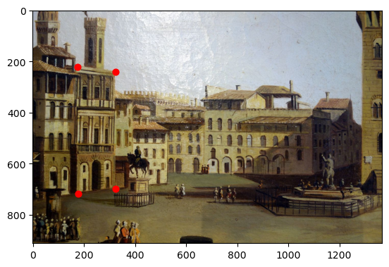
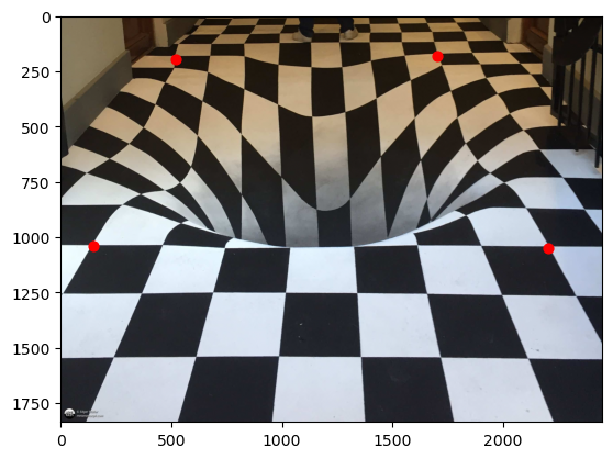
Then, for each image, I mapped the four corners I labelled to the four corners of a rectangle of proper dimensions, and solved for the inverse homography. I solved for the inverse so that I could iterate over every pixel (using efficent numpy code) of the target shape and avoid any holes in the image. Using this mapping, I populated the target range with pixels from the source image.
This is how I rectified the skull from Holbein's painting, and also produced the following results:
Interestingly, you can see that the floors of the building are not level with each other, which I did not notice in the original image. I guess it worked!
Unfortunately, creating a mosaic image isnt as simple as overlapping the areas they have in common to get a larger images. This is because the images were taken at different angles, and need to be transformed onto the same plane as each other.
Therefore, every image must be rectified to its adjacent image using a homography, using the same labelling tool as earlier to label corresponding points:

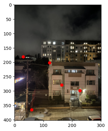
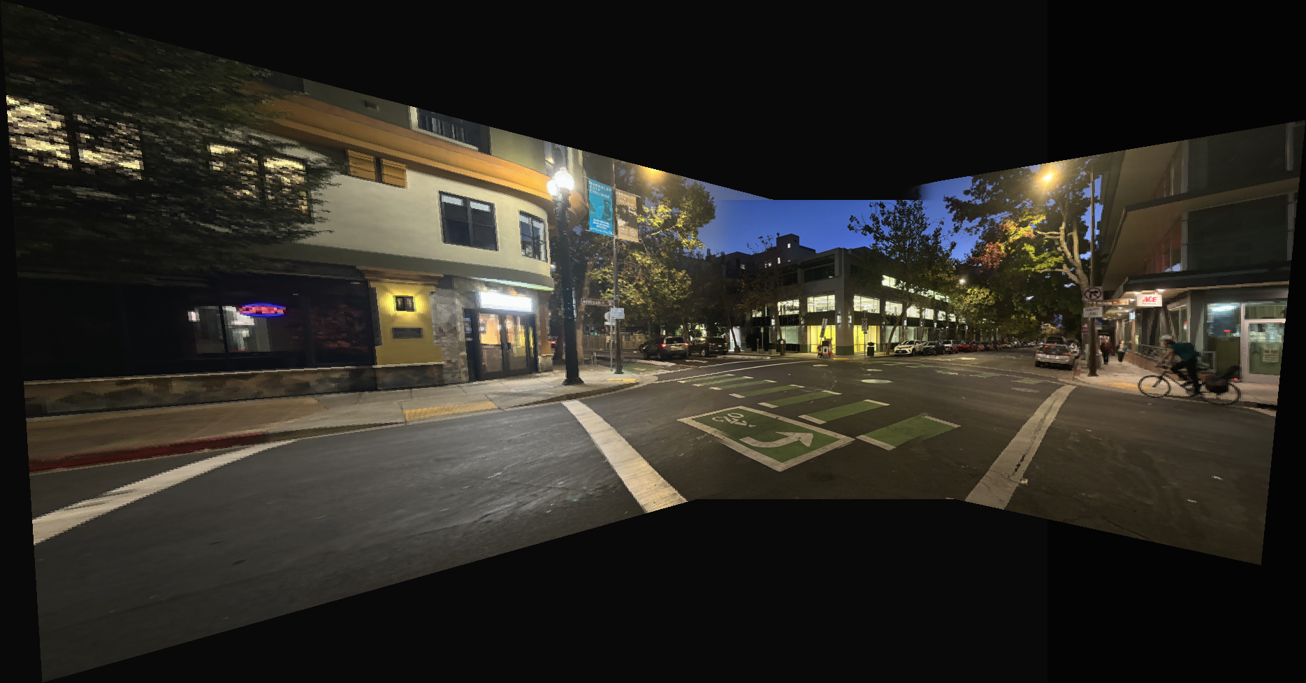
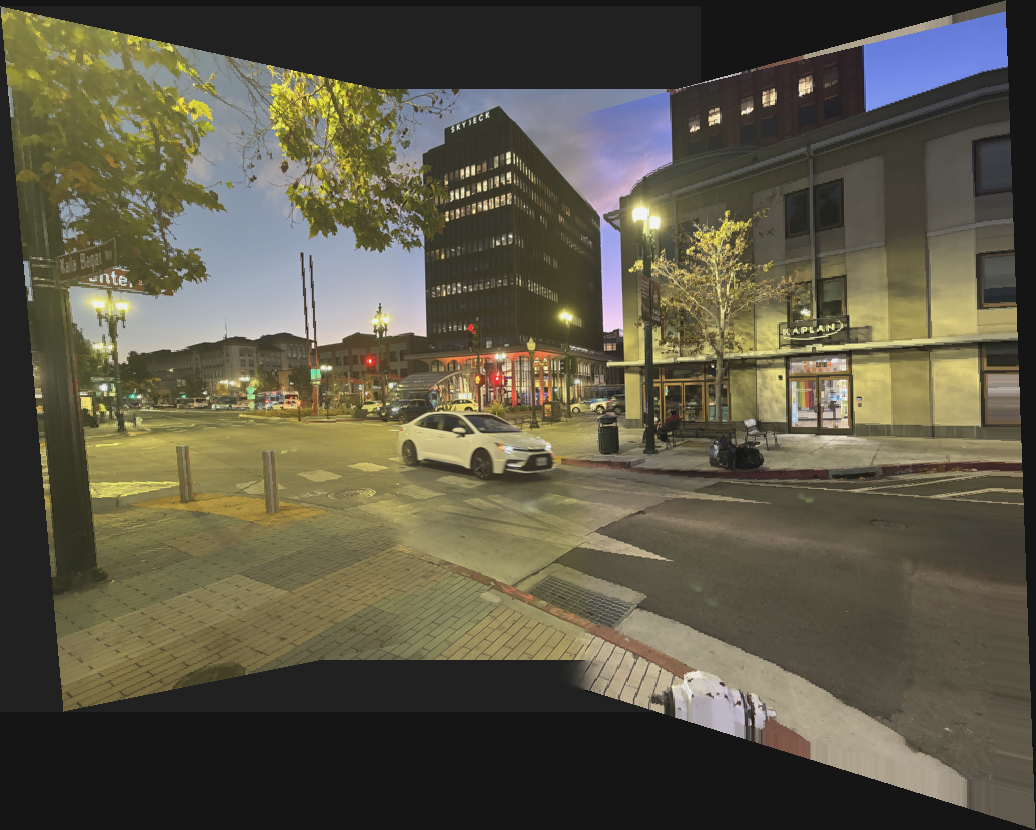
After the points are gathered, we transform both images onto the same image array, using a similar process as when we did rectification. Crucially, we need to determine the center of intersection and perform a laplacian blending, just like in project 2. Without this blending, there would be a sharp edge between the two images, due to the exposure settings that a cell phone's camera applies automatically.
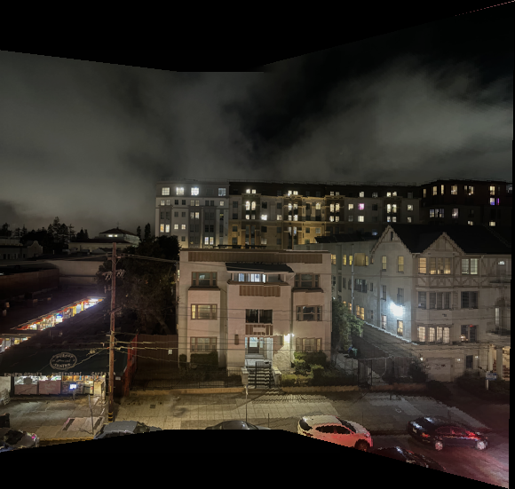
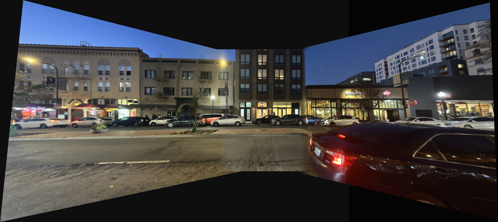
This transformation and blending process is repeated for each image in the mosaic. Here are my final results for the three sets of images:
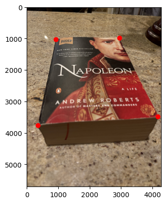
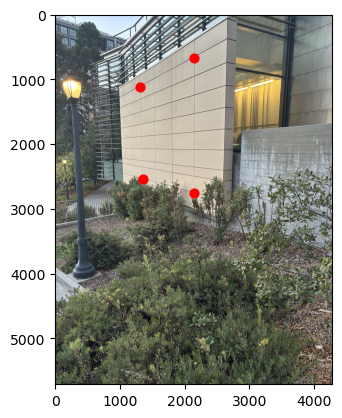
Another thing we can do is transform parts of an image to match the perspective of another. In this case, neither area is rectangular, and I used my labelling tool from above to map a non-rectangular area to another:
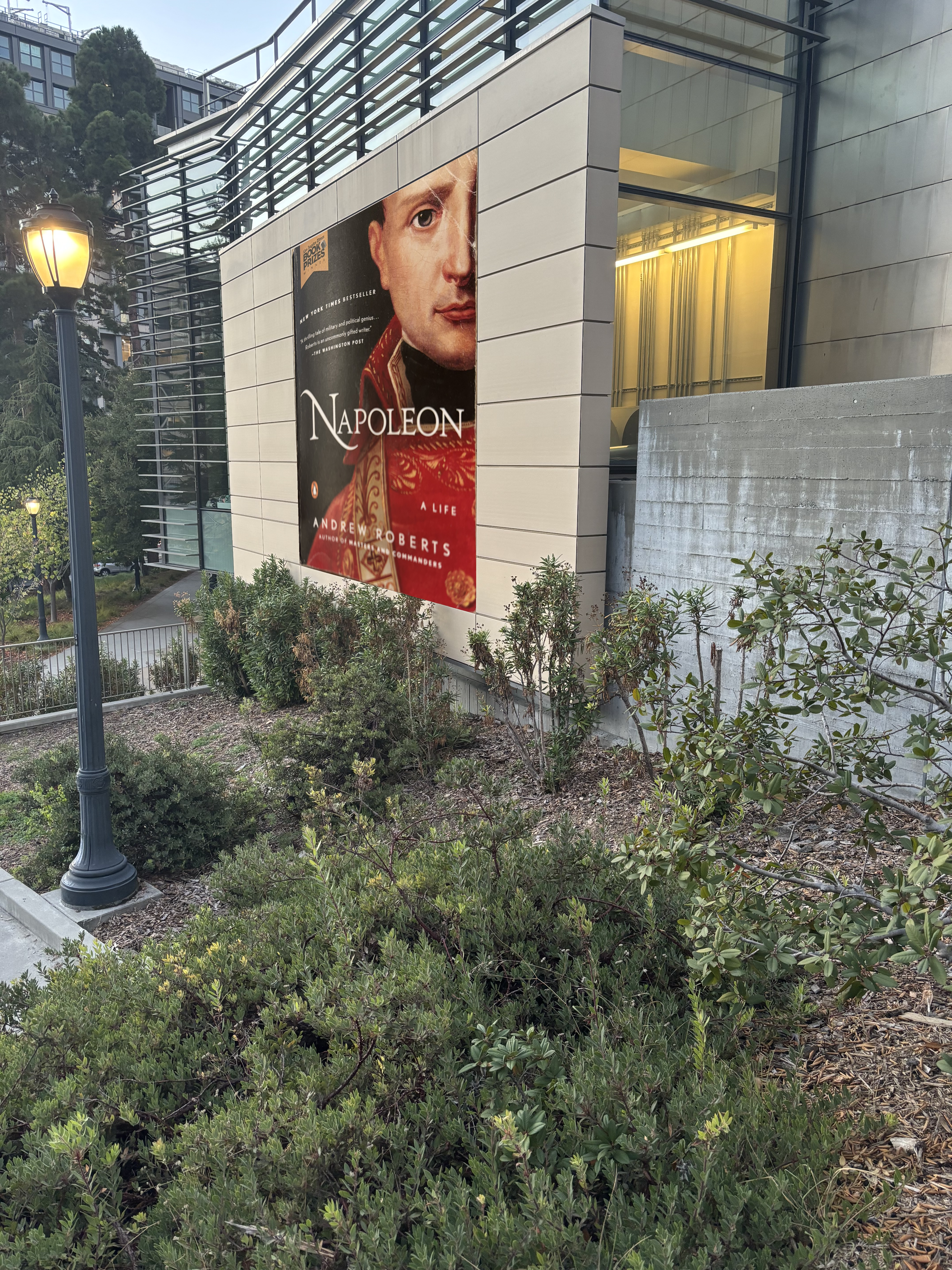
This was a simple, yet suprisingly effective technique. I expirimented with gaussian blending, however it is better to not use it in this case as you do not want the "poster" to blend into the wall. Instead, I chose the two pictures intentionally so that the light from the lamp appears to be reflecting off of the "poster", which also has a bit of glare.
Now, the task is to have the computer properly determine correspondences between overlapping images, without us having to do it manually.
In part 1 when we wanted to indicate correspondences, the easiest places to label were corners. It turns out that is similar for computers - corners are easy to identify across seperate images by using Harris Corners. The main idea is that we can apply a convolution to every pixel on the image (other than the edges, where the convolution is ill defined). This will give us a scalar value for each pixel, telling us how "cornery" it is.
One way to use this value is to just take the say, first 50 values:
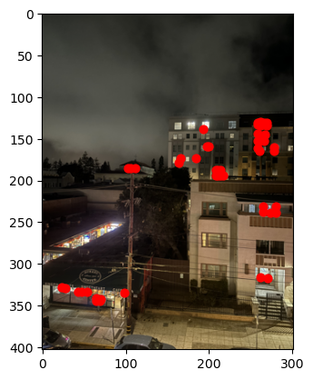
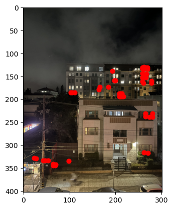
However, there is an issue with just taking the first n strongest Harris Corners. Often, they are distributed disproportionately over the image: in this case, most of them are on buildings, and almost none are in the sky. This is not ideal for our end goal of calculating a homography.
So we have two competing interests: 1, we want our corners to be strong, and 2, we wants them to be well distributed. To try and balance these interests, we use Adaptive Non-Maximal Supression (ANMS) which takes into account both the Harris strength of the pixel and a new quantity called a "supression radius" which is calculated based on a points distance from a sufficently stronger corner. The complete algorithm is described in the paper, but the result is that it gives us a much more homogenous distribution of corners, which are still strong relative to their neighboring corners:

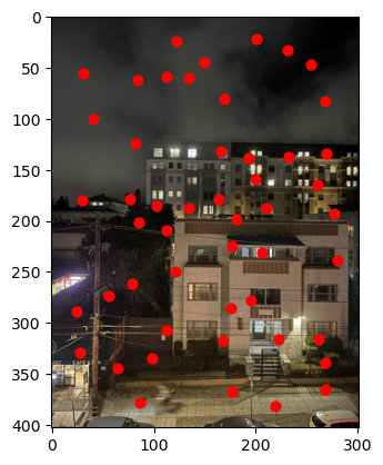
We have the corners in each image. Alone, this is not useful to us as the coordinates of corners in the image give us very little information. We need a way of featurizing the image around these points, so that we can match corners between the images.
Following the paper, we do the following steps:
1) Take the 40 x 40 area of pixels (of which each corner is the center)
2) Denorm and standardize Each 40 x 40 matrix
3) Downscale to 8 x 8
4) Vectorize the patch into a 192 dimension vector (8 x 8 x 3 color channels). I think the paper used greyscale features, but I decided to do it this way and it was effective.
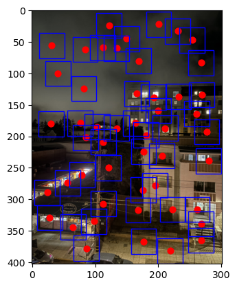
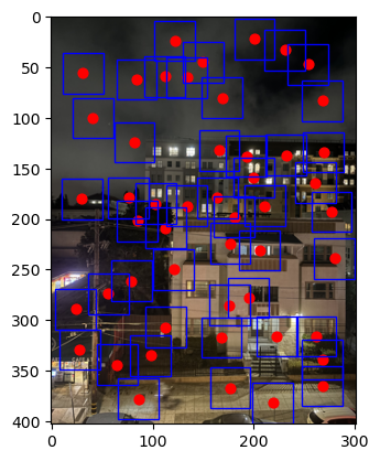
Now that we have a vector representation of the features, we can worry about actually creating pairs of corners, which we beleive correspond to the same real world locations between images.
To do this, we will use Lowe Thresholding. The idea is that, for all valid featue correspondences between image 1 and 2, the closest neighbor for a feature in image 1 to a feature in image 2 should be much closer than the second nearest neighbor. This is not true for invalid correspondences, where the second nearest neighbor may only be slightly further away than the first nearest neighbor. Intuitively, this is because in most cases there is exactly 1 place in each image that is exactly the same as in the other image.
So, by finding the 1st and 2nd nearest neighbors, we can only retain the points that have a sufficently low ratio. For example, in the below images, my cutoff ratio was .25, meaning that the first nearest neighbor had to be 4x closer than the second to be considered a valid correspondence.
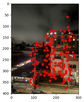
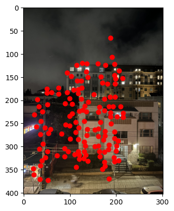
As a side note, I used numpy based linear algebra to calculate the optimal neighbors, as fancy algorithms will suffer from the law of large numbers, making numpy the most efficent solution in practical terms.
As you can see, most points that appear in one image also appear in the other. Notice how only the overlapping area of the image has points.
Though Lowe Thresholding is pretty good at weeding out false correlations, the situation in the last section was pretty ideal. In practice, I found that in most images, I had to increase the cutoff from .25 to .4, which allowed in more false correlations. Even if the .25 cutoff lets in a sufficent amount of points, if even one of them is incorrect, it can throw off the homography calculation completely. Therefore, we need another layer of protection against outliers.
The Random Sample Consensus (RANSAC) algorithm is a method of picking points from a group that well represent the majority of the points. It goes as follows:
1) Pick 4 pairs from the points identified by Lowe Thresholding
2) Calculate the homography using this subset
3) Calculate how many of the transformed first points are within a specified epsilon radius from the actual second point
4) Repeat this process many times, and calculate the final homography based on the biggest group of inliers. This group is unlikely to have outliers, and will produce a robust homography.
In practice, I found using RANSAC with 1000 iterations usually was very robust even against a significant portion of the points being false matches! I eventually tuned the pipeline so they could almost always match images, even if only a small area was overlapping.

Manual Stitching
Automated Pipeline
Automated Pipeline
Automated Pipeline
Automated Pipeline